LLM pretraining for generalists
What and why
This is the post I would've liked to read when I started learning about LLMs. It assumes a general familiarity with software engineering and high school math. Hopefully, by the end of it, you will have a deep enough understanding of LLMs that they no longer feel like a magical black box.
Training a modern LLM has two broad stages. Pretraining teaches a base model to predict the next token across a large text corpus, producing most of its underlying capabilities. Post-training then shapes those capabilities so they are easier to steer and use. This post focuses on pretraining and the resulting base model.
I'll start with a brief history of the machine-learning ideas that led to LLMs, look at GPT-2 at a high level, follow text through the model, take attention and learning apart, explain how GPT-2 generates text, and finally examine state-of-the-art (SOTA) models using GPT-2 as a reference point.
History of language models
Like all complex systems, LLMs evolved from a sequence of simpler ideas. A useful thread begins with the weighted sum: combine several inputs, give each one a learned importance, and add a bias. Perceptrons used this calculation to classify inputs; multilayer perceptrons (MLP) stacked it to represent nonlinear patterns; later architectures adapted it to sequences and, eventually, attention. Following that progression will take us from a single linear model to GPT-2State-of-the-art LLMs still build on the same underlying concepts, so understanding GPT-2 remains as relevant as ever; its public code and weights also make it practical to study firsthand..
- $x$ is the vector of input features.
- $w$ is the vector of weights, one for each input feature; the superscript $\mathsf{T}$ transposes $w$ so $w^\mathsf{T}x$ computes the dot product.
- $b$ is the bias, or the model's starting point before considering the features.
- $y$ is the prediction.
This equation is a linear model: it maps a collection of inputs to one output. For example, if the model predicts a house price, the inputs might be size, number of bedrooms, and distance to the nearest school. If the baseline price is \$80,000, the bias might represent that starting point. The weights then adjust the prediction: square footage may push the price up, distance from a school may push it down, and so on. Learning means finding useful values for those weights and the bias from examples.
A perceptronSee Frank Rosenblatt, “The Perceptron: A Probabilistic Model for Information Storage and Organization in the Brain” (Psychological Review, 1958). builds on the weighted sum plus bias with two innovations. First, it passes the result through a threshold function, turning the continuous score into a binary prediction and making the calculation useful for practical classification tasks:
Second, the perceptron helped establish a central machine-learning paradigm: learn parameters from labeled examples instead of programming classification rules by hand. Given the correct label $y$ and the perceptron's prediction $\hat{y}$, it computes the error $e = y - \hat{y}$ and updates each weight and the bias:
Here, $\eta$ is a chosen learning rate. A correct prediction makes $e = 0$, so nothing changes. After a mistake, each weight changes in proportion to the error and its corresponding input value, while the bias changes by the scaled error alone. Repeating this process over labeled examples lets the perceptron learn its decision rule from data.
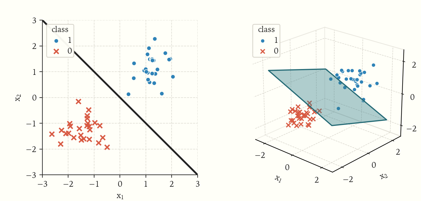
Linear models that rely on $w^\mathsf{T}x + b$, like the perceptron, have many limitations. First, they can represent only a single linear decision boundary: a line in two dimensions, a plane in three, or a hyperplane in higher dimensions, as shown in Figure 1. This can work well when a roughly linear boundary separates the classes, but it cannot capture more complex, nonlinear structure. Second, a linear model learns weights over the features it is given; it does not learn a better representation of the raw data. Useful features must therefore be designed or extracted before the model sees them, and those features are not always obvious in advance.
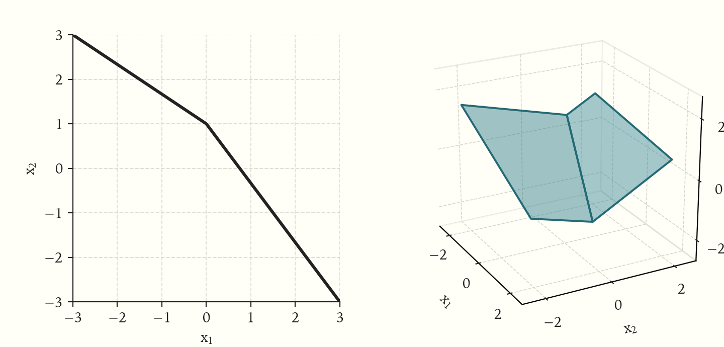
A multilayer perceptron (MLP) addresses both limitations by stacking many weighted sums and placing nonlinear activation functions between them. The activations introduce bends into a line in two dimensions, a plane in three, or a hyperplane in higher dimensions, as shown in Figure 2. By combining many such bends, an MLP can learn flexible, nonlinear decision boundaries. Its hidden layers also learn intermediate representations of the input, and greater depth lets later layers build increasingly complex features from simpler ones.
A two-layer MLP can be written as:
- $x$ is the input vector.
- $f$ is the nonlinear activation function.
- $y_1$ is the first layer's output vector.
- $y_2$ is the MLP's final output vector.
- $W_1$ and $W_2$ are weight matricesThe uppercase $W$ and vector $b$ describe the parameters of an entire layer. In contrast, lowercase $w$ and scalar $b$ describe one weighted sum, as used by a single neuron..
- $b_1$ and $b_2$ are bias vectors.
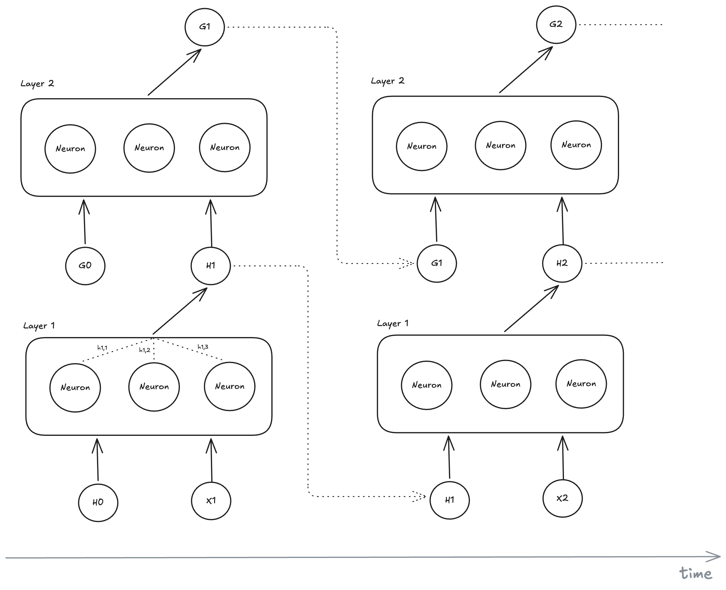
A standard MLP has no built-in memory of earlier inputs, making it a poor architectural fit for sequential or time-dependent data. A recurrent neural network (RNN)See nbro, “Where can I find the original paper that introduced RNNs?” (Artificial Intelligence Stack Exchange, 2020). solves this issue by processing a sequence one step at a time and carrying a hidden state forward, as shown in Figure 3. At step $t$, the recurrent layer combines the current input $x_t$ with the previous hidden state $H_{t-1}$. It applies learned weights and a bias, then passes the result through an activation function:
The resulting hidden state $H_t$ is a compressed running summary of the sequence processed so far.
RNNs were a natural fit for language because they process tokensFor text, a token is to an LLM roughly what a word is to a person: the basic unit it reads and predicts. Depending on the tokenizer, it can be a whole word, part of a word, an individual character, punctuation, whitespace, or a byte fragment. in order while carrying context forward. Machine translation became an obvious test case because both the source and translated sentences are sequential, and collections of paired translations provided training data. A common architecture used two RNNs side by sideSee Kyunghyun Cho et al., “Learning Phrase Representations using RNN Encoder-Decoder for Statistical Machine Translation” (arXiv, 2014), and Ilya Sutskever, Oriol Vinyals, and Quoc V. Le, “Sequence to Sequence Learning with Neural Networks” (NeurIPS, 2014)., as shown in Figure 4. The first one, the encoder, reads the source sentence one token at a time and compresses it into a hidden-state representation, while the second one, the decoder, generates the translated sentence one token at a time while conditioned on the encoder's final state.
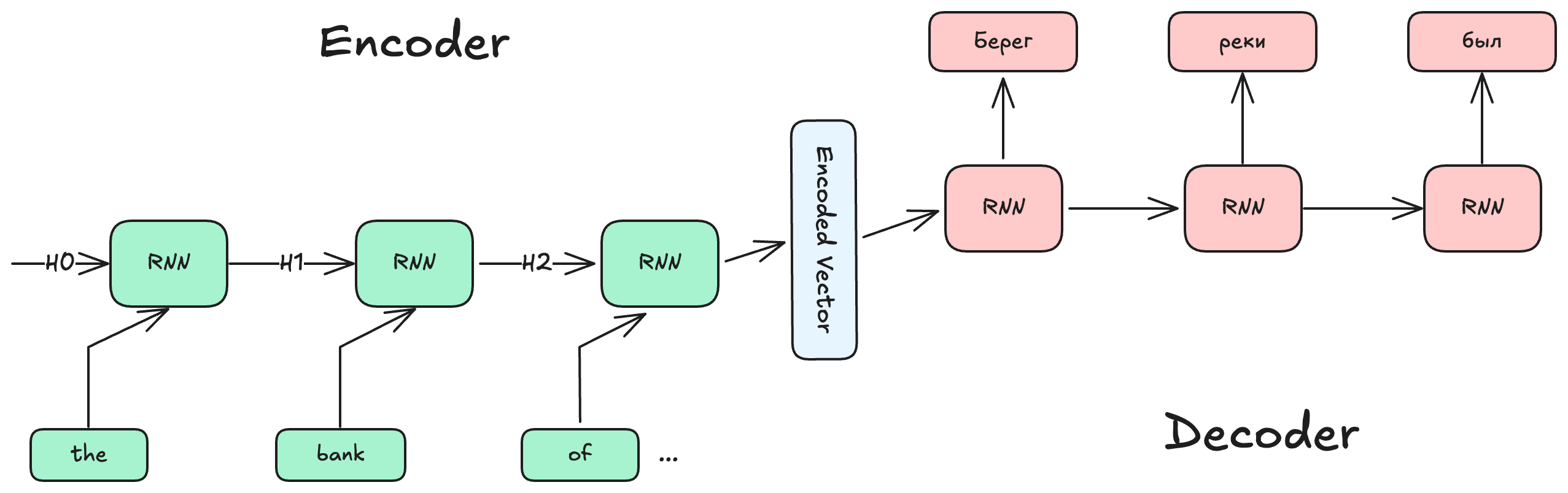
This design has three important limitations. First, each hidden state depends on the previous one, so training cannot be fully parallelized across the sequence. Second, the encoder's final state has to carry everything the decoder may need, creating a fixed-size compression bottleneck. Third, information from early tokens has to survive many recurrent steps, making long-range patterns difficult to learn.
A convolutional neural network (CNN) builds on the same weighted sum plus bias used by each MLP neuronThink of a neuron as a single unit inside an MLP layer. It computes a weighted sum plus bias, then applies an activation function: $y = f(w^\mathsf{T}x + b)$.. Instead of connecting every input to every neuron, a CNN filter applies that calculation to one small local region at a time and reuses the same weights as it slides across the input.
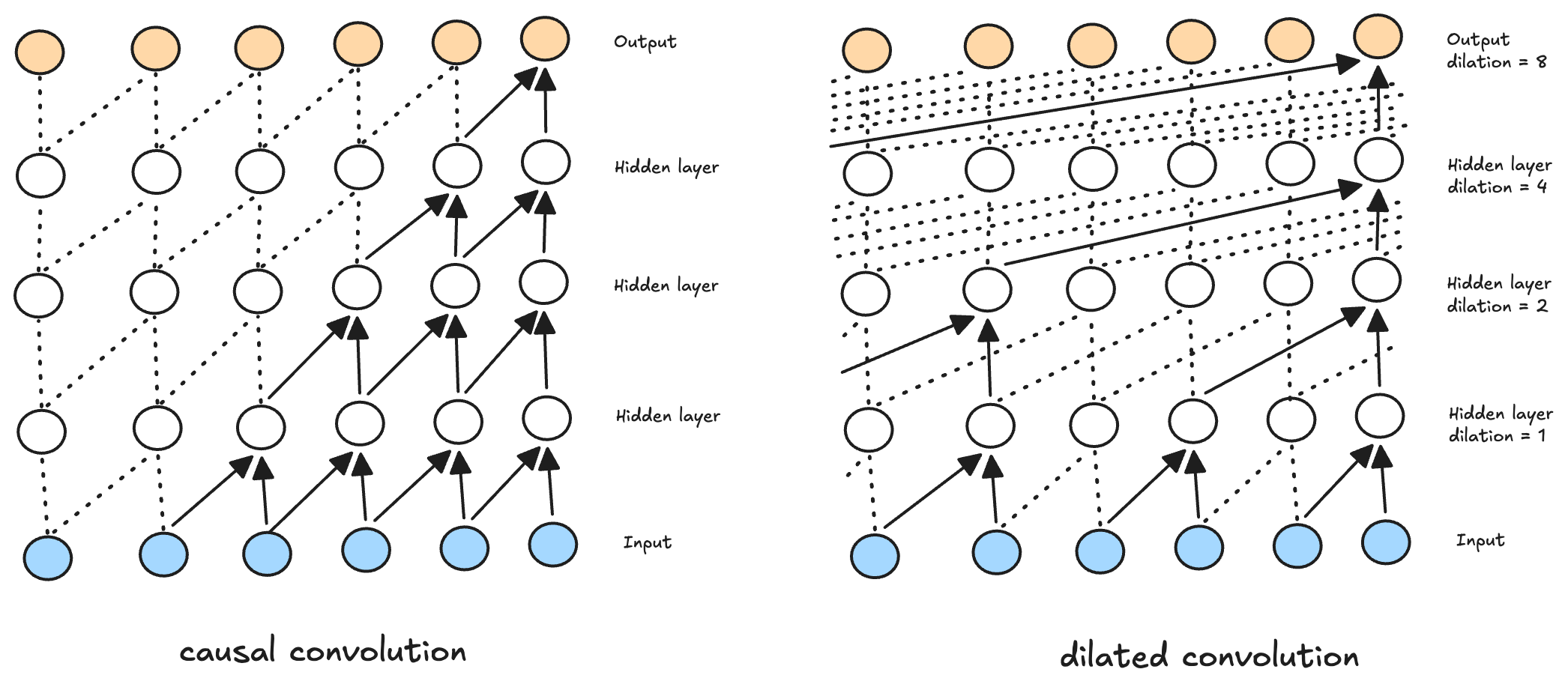
Sequence CNNs applied the same idea along one-dimensional sequences. Unlike an RNN, a convolution applies the same local filter at every position, allowing all positions to be processed in parallel during training. As shown in Figure 5, autoregressiveAutoregressive generation means the model predicts one token at a time, then feeds each newly generated token back in as part of the input sequence for the next prediction. models such as WaveNet for raw audio and ByteNet for character-level language modeling and translation used causal (or masked) convolutions so no output depended on future positions, and dilated convolutions so deeper layers could reach farther back without a long chain of recurrent stepsSee Aaron van den Oord et al., “WaveNet: A Generative Model for Raw Audio” (arXiv, 2016), and Nal Kalchbrenner et al., “Neural Machine Translation in Linear Time” (arXiv, 2016).. This made training more parallel and gave distant context a shorter path through the network, although autoregressive generation still proceeded one element at a time.
Building on the encoder-decoder RNNs, Bahdanau attentionSee Dzmitry Bahdanau, Kyunghyun Cho, and Yoshua Bengio, “Neural Machine Translation by Jointly Learning to Align and Translate” (arXiv, 2014). let each decoder step compute which encoder steps are most relevant for the next translated token. The TransformerSee Ashish Vaswani et al., “Attention Is All You Need” (NeurIPS, 2017). kept the overall architecture but dispensed with recurrence and convolutions entirely, making attention—both self-attention within a sentence or its translation, and encoder-decoder attention across them—the central mechanism for exchanging information between sequence positions. See the Attention section for a more detailed, visual treatment of attention in general and the Transformer in particular.
Perceptron through attention is a series of answers to one question: how should a network move information? MLPs mix features within one input, convolutions reuse the same local rule across positions, RNNs carry a compressed state forward, and attention draws dependencies between positions. A Transformer combines attention with MLPs, then repeats the pair. GPT-2 is, in that sense, not a wholly new machine but a particular arrangement of the ideas we have just followed.
GPT-2 in one picture
This section shows GPT-2 as a whole; the next follows text through it step by step. Throughout this walkthrough, I make several simplifying assumptions, including omitting the batch dimension from the shapes of tensors that pass through the model ($4 \times 768$ instead of $b \times 4 \times 768$).
The original Transformer used an encoder-decoder architecture for language translation. However, subsequent research showed that isolating and scaling just one of these components yielded superior results for targeted tasks. Encoder-only models (eg BERTSee Jacob Devlin, Ming-Wei Chang, Kenton Lee, and Kristina Toutanova, “BERT: Pre-training of Deep Bidirectional Transformers for Language Understanding” (arXiv, 2018).) look at both left (past) and right (future) tokens to excel at text classification tasks. Meanwhile, decoder-only models (eg GPTSee Alec Radford et al., “Improving Language Understanding by Generative Pre-Training” (OpenAI, 2018).) rely on causal masking to look only at past tokens, autoregressively predicting the next token to excel at generative tasks.
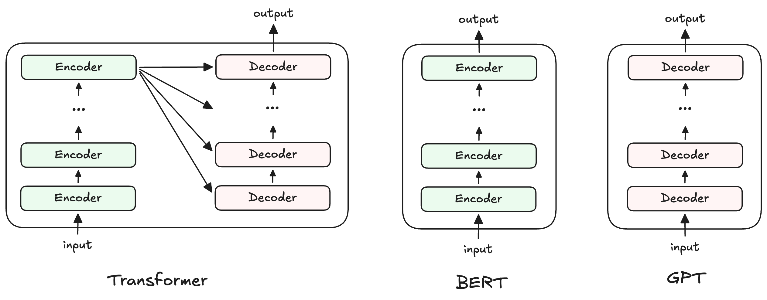
GPT-2 has four sizes: Small, Medium, Large, and XLSee Alec Radford et al., “Language Models are Unsupervised Multitask Learners” (OpenAI, 2019), and OpenAI, “GPT-2: 1.5B release” (OpenAI, 2019)., with progressively more decoder blocks ($L$ in the table below) and wider hidden representations. I will focus on GPT-2 Small (GPT-2 from here on), which is small enough to experiment with on a regular laptop and is depicted in Figure 7.
| Parameter | GPT-2 Small | GPT-2 Medium | GPT-2 Large | GPT-2 XL |
|---|---|---|---|---|
| Layers ($L$) | 12 | 24 | 36 | 48 |
| Hidden size ($d_{model}$) | 768 | 1,024 | 1,280 | 1,600 |
| Attention heads ($A$) | 12 | 16 | 20 | 25 |
| Head dimension ($d_{model}/A$) | 64 | 64 | 64 | 64 |
| Feed-forward size | 3,072 | 4,096 | 5,120 | 6,400 |
| Vocabulary size | 50,257 | 50,257 | 50,257 | 50,257 |
| Context length | 1,024 | 1,024 | 1,024 | 1,024 |
| Parameters | ~124M | ~345M | ~762M | ~1.5B |
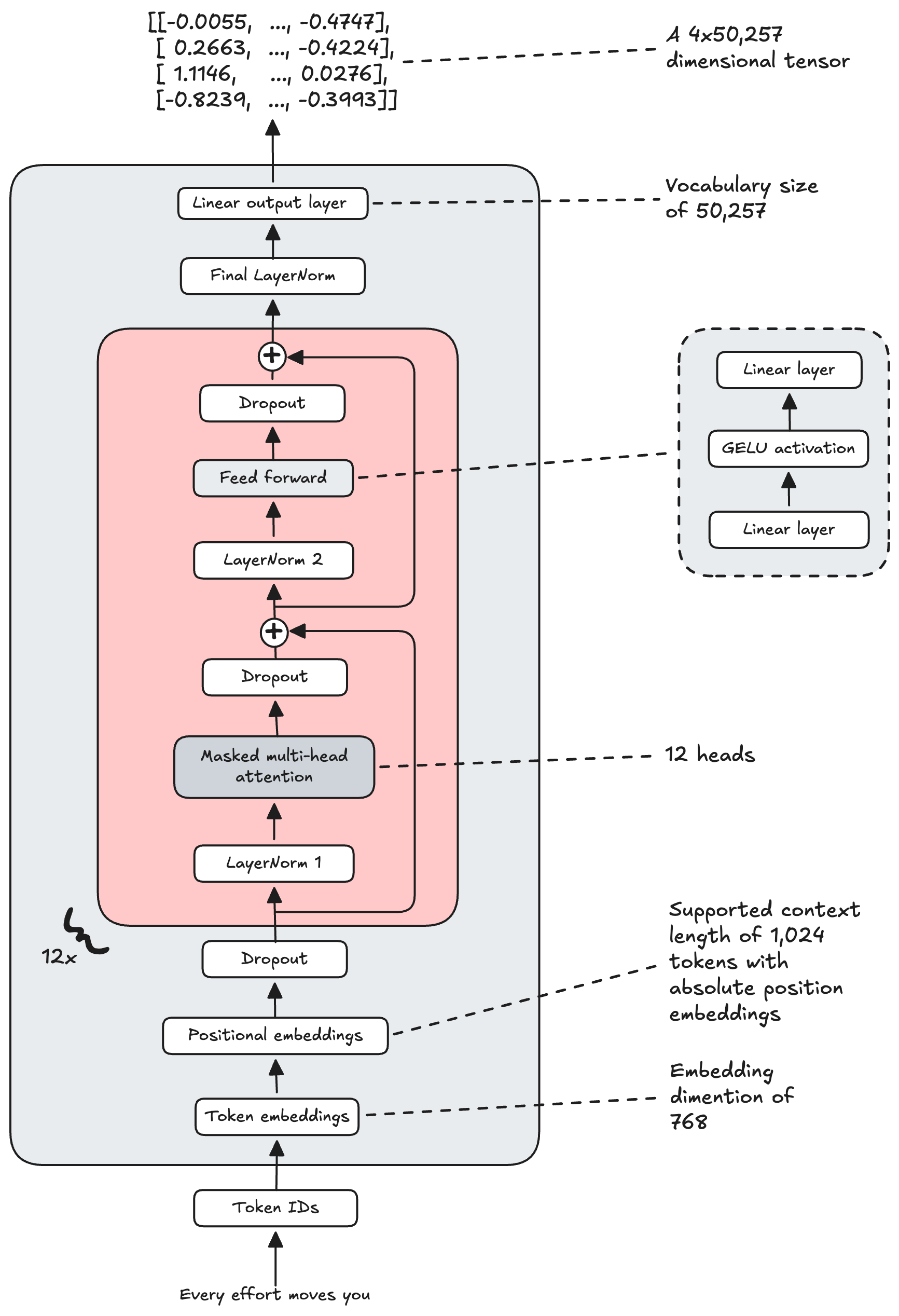
The core of GPT-2 is a stack of 12 sequential decoder blocks (red in Figure 7). Each block has two main components: masked multi-head self-attention and a feed-forward network (FFN). In the attention module, each token position computes which previous positions, including itself, it should attend to. GPT-2 uses 12 attention heads; each head has its own learned projections and works in a 64-dimensional subspace of each token’s 768-dimensional feature vector.
Unlike attention, the FFN operates independently on each position. By this point, attention has already brought contextual information into each token representation, so the FFN can transform that representation by combining its internal features. The GELUSee Dan Hendrycks and Kevin Gimpel, “Gaussian Error Linear Units (GELUs)” (arXiv, 2016). activation acts like a smooth nonlinear gate, allowing some feature patterns to pass through more strongly than othersSee Ivan Arcuschin, “MLPs in Transformers” (Learn MI, 2026)..
Following text through GPT-2
This section follows Figure 7's four-token example through the training-time forward passThe forward pass uses the model's current weights and biases to make predictions. During training, the backward pass updates those weights and biases based on the prediction error..
After tokenization, the four token IDs are turned into token embeddings and combined with position embeddings, producing a tensor with shape $4 \times 768$. That tensor enters the stack of 12 decoder blocks, shown in red in Figure 7, and comes out of each block with the same $4 \times 768$ shape. Within each decoder block, attention moves information between rows, while the FFN processes each row individually. After the final block and LayerNorm, the linear output layer—the topmost rectangle in Figure 7—projects the tensor into $4 \times 50{,}257$ logits.
The four rows correspond to four predictions: the first is based only on “Every,” the second on “Every effort,” and so on. Each of the 50,257 columns corresponds to a unique token in the GPT-2's vocabularyThe vocabulary is the fixed set of token IDs that GPT-2 can receive or predict. Its size is chosen explicitly, and its entries are produced when the tokenizer is trained..
Text becomes token IDs
The path shown in Figure 7 begins at the bottom with tokenization, which converts the text into indices in the vocabulary called token IDs: $[6109, 3626, 6100, 345]$. For example, 6100 represents “ moves,” including the leading space.
Before GPT-2 itself is trained, its tokenizer uses byte-level Byte Pair Encoding (BPE)BPE is a compression algorithm adapted for language-model tokenization. See Rico Sennrich, Barry Haddow, and Alexandra Birch, “Neural Machine Translation of Rare Words with Subword Units” (ACL, 2016). to learn two things from training text: a fixed vocabulary and an ordered list of byte-pair merges. Tokenizer training begins with 256 base tokens, one for each possible byte value, then repeatedly merges the most frequent adjacent pair into a new token. After 50,000 such merges, the 256 base tokens, 50,000 merge-created tokens, and special <|endoftext|> token form GPT-2's fixed vocabulary of $256 + 50{,}000 + 1 = 50{,}257$ entries. The tokenizer saves the merge order and applies it later when encoding new text.
Once the vocabulary and merge rules are fixed, encoding new text begins with a regex pattern that splits it into smaller contiguous chunks such as words, contractions, numbers, punctuation, and whitespace. These chunks are called pre-tokens, and their boundaries prevent BPE from merging across character categories. The example becomes ['Every', ' effort', ' moves', ' you'].
Next, each pre-token is encoded as UTF-8 bytes, and those bytes are mapped reversibly to the Unicode symbols used by GPT-2's BPE implementation. The tokenizer applies the stored merge rules within each pre-token until no learned rule applies. In the main example, every pre-token remains intact because its complete byte sequence appeared often enough during tokenizer training to become a token. Longer or less common pre-tokens may be divided: for example, “ uncharacteristically” becomes [' un', 'character', 'istically']. Finally, the tokenizer looks up each resulting token in the fixed vocabulary and returns its token ID. The complete example is:
text      : Every effort moves you
pre-tokens: ['Every', ' effort', ' moves', ' you']
tokens    : ['Every', ' effort', ' moves', ' you']
token ids : [6109, 3626, 6100, 345]
Token IDs become vectors
At this point, raw text has become token IDs. The next step is to convert those token IDs into token embeddingsAn embedding is a vector representation of a token that places it in a high-dimensional space. Tokens with similar meanings are closer together in this space, allowing the model to use semantic and syntactic similarities and differences. In GPT-2, each token embedding starts as a randomly initialized vector of 768 numbers and is learned during training.. This is done by first having GPT-2 randomly initialize embeddings for all tokens at once and store them in a token embedding table $W_E$ with shape $50{,}257 \times 768$, then looking up individual embeddings based on token ID. For example, “ effort” has its embedding stored in the 3626th row of $W_E$.
A token embedding by itself does not contain position information: the same token ID always retrieves the same row from $W_E$. Consider the token sequences “the dog chased the cat away” and “the cat chased the dog away”: although their token order differs, each token receives the same embedding in both sequences. GPT-2 therefore adds a position embedding to each token embedding. These position embeddings are randomly initialized all at once and stored in a learned lookup table $W_P$ with shape $1{,}024 \times 768$, where 1,024 is GPT-2's chosen context length. At position $t$, GPT-2 looks up the token's absolute-position vector and adds it to the token vector, so the input embeddingThe input embedding is the vector fed into the Dropout box and then into the decoder blocks, shown as the red box in Figure 7. is $W_E[\text{token ID}] + W_P[t]$. When later decoder layers update the representation for “away,” they can use the different position-aware representations of “dog” and “cat” to determine which animal chased the other.
Vectors pass through dropout and LayerNorm
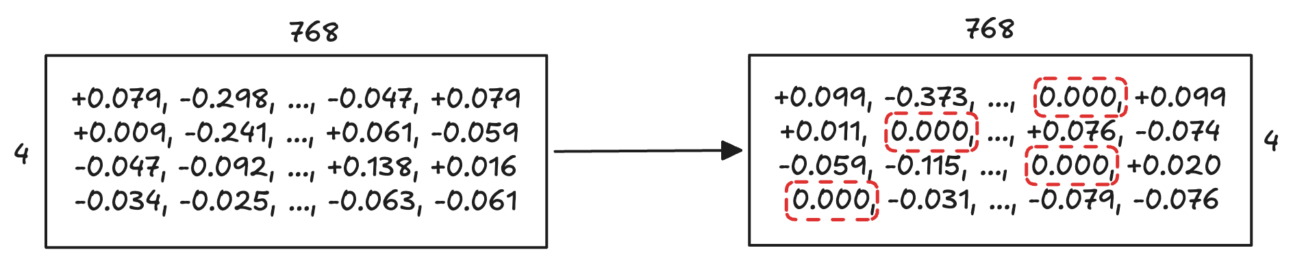
Before the input embeddings enter the decoder blocks, GPT-2 applies dropoutSee Nitish Srivastava, Geoffrey Hinton, Alex Krizhevsky, Ilya Sutskever, and Ruslan Salakhutdinov, “Dropout: A Simple Way to Prevent Neural Networks from Overfitting” (JMLR, 2014)., a technique where some percentage of the 4 × 768 input-embedding cells are ignored, as shown in Figure 8, effectively dropping them out. It helps reduce overfittingOverfitting describes a scenario where a model learns the training data too perfectly, including its noise, quirks, and outliers, causing it to perform exceptionally well on seen data but fail to accurately predict unseen data. by ensuring the model does not become overly reliant on any specific set of hidden-layer units. As part of dropout, the remaining values in the input embeddings are scaled up by a fixed factor to compensate for the reduction in active elements; for example, when the drop rate is 20%, the fixed factor is $1 / (1 - 0.2) = 1.25$. Dropout is disabled after training.
LayerNorm then recenters and rescales each token vector's features to have mean 0 and variance 1, then applies element-wise learned scale ($\gamma$) and shift ($\beta$) parametersSee Jimmy Lei Ba, Jamie Ryan Kiros, and Geoffrey E. Hinton, “Layer Normalization” (arXiv, 2016)..
Setting each token vector's mean to 0 and variance to 1 gives the next sublayer a more stable baseline by keeping the values on a predictable scale and dampening unusually large ones. Then applying the learned scale and shift gives the model a way to undo some potential damage from strict standardization by restoring useful feature-specific scale or offset. See Figure 9 and the code block below to follow the red-highlighted scalar through the mean-0, variance-1 standardization step.
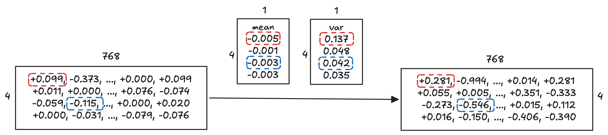
x[0,0] = 0.099
mean[0,0] = -0.005
var[0,0] = 0.137
std ≈ sqrt(0.137 + 0.00001) ≈ 0.370

norm_x[0,0] ≈ (0.099 - (-0.005)) / 0.370
            ≈ 0.104 / 0.370
            ≈ 0.281
Vectors pass through attention and residual connections
The normalized vectors now enter masked multi-head attentionThe next section takes attention apart from first principles.. Attention's job is to mix information between token positions: each token vector can retrieve information from earlier tokens and decide which ones matter for its next representation. After attention, GPT-2 applies dropout again to the attention output.
GPT-2 then adds the vectors that entered the decoder block back to the attention output. The first plus sign inside the decoder block in Figure 7 marks this addition; the second marks the same kind of operation after the FFN. Both are residual connectionsSee Kaiming He, Xiangyu Zhang, Shaoqing Ren, and Jian Sun, “Deep Residual Learning for Image Recognition” (arXiv, 2015).. A residual connection means the block does not replace a token vector outright. It keeps the original vector, lets a sublayer compute an update, and then adds that update back. This makes deep networks easier to train by giving gradients direct additive paths through the network during the backward pass, allowing them to bypass one or more sublayer transformations. After this addition, the vectors are normalized again before entering the FFN.
Vectors pass through the feed-forward network
The FFN is a two-layer MLP that transforms each contextualized token vector independently. It first projects each 768-dimensional row to 3,072 dimensions (a 4× up-projection), producing a $4 \times 3{,}072$ tensor:
The expanded vector then passes through GELU. As in the MLP introduced earlier, the nonlinear activation function lets the FFN learn nonlinear patterns, while the 4× expansion gives it a richer representation space in which to detect and combine them before projecting the result back to 768 dimensions:
Finally, a second linear layer projects the activated vector back down to the original model dimension:
This FFN contains about two-thirds of each decoder block’s parameters, so most of the block's learnable capacity sits in the FFN. During training, the first layer learns pattern detectors for contextualized token vectors while the second layer learns what information should be written into the output token vector when that pattern is detected. This gives the FFN a soft key-value memory interpretationSee Mor Geva, Roei Schuster, Jonathan Berant, and Omer Levy, “Transformer Feed-Forward Layers Are Key-Value Memories” (EMNLP, 2021).: the detectors act as keys, and their output vectors act as values. Several detectors can activate at once, so the FFN combines their output vectors according to how strongly each detector activates.
After the FFN, dropout is applied again and another residual connection adds the attention-updated vectors back to the FFN output, as shown in Figure 7. The same sequence repeats through all 12 blocks.
Final vectors become next-token logits
After the 12 decoder blocks, GPT-2 produces one 768-dimensional output row for each 768-dimensional input row. Each output row is an enriched version of its corresponding input token representation, incorporating information from the token itself and all earlier tokens in the sequence. Preserving this one-to-one mapping is an explicit design choice.
Those output vectors are normalized one more time. A final linear projection then turns each row into 50,257 scores called logits:
Softmax converts each row's logits $z_i$ into probabilities:
Those probabilities are then compared with the actual next tokens to evaluate the predictions and calculate the loss for this forward pass.
Attention
With GPT-2 now examined at both the architectural and component levels, let's zero in on its central context-mixing mechanism: attention. Consider the sentence “The river bank was muddy.” The earlier word “river” makes “bank” more likely to mean a slope of land than a financial institution. Attention turns that kind of contextual dependence into a computation: it lets each token's representation selectively draw on earlier tokens in the sequence.
An early version of this idea appeared in a 2014 paper on neural machine translationSee Dzmitry Bahdanau, Kyunghyun Cho, and Yoshua Bengio, “Neural Machine Translation by Jointly Learning to Align and Translate” (arXiv, 2014).. Building on the recently proposed encoder-decoder architecture, the paper introduced an extension: instead of encoding a whole input sentence into a fixed-length vector, the encoder produced a sequence of vectors. The decoder then (soft-)searched over positions in the source sentence to find where the most relevant information was concentrated. In this setting, attention acted as a way to learn a linguistically plausible (soft-)alignment between the source sentence and its translation.
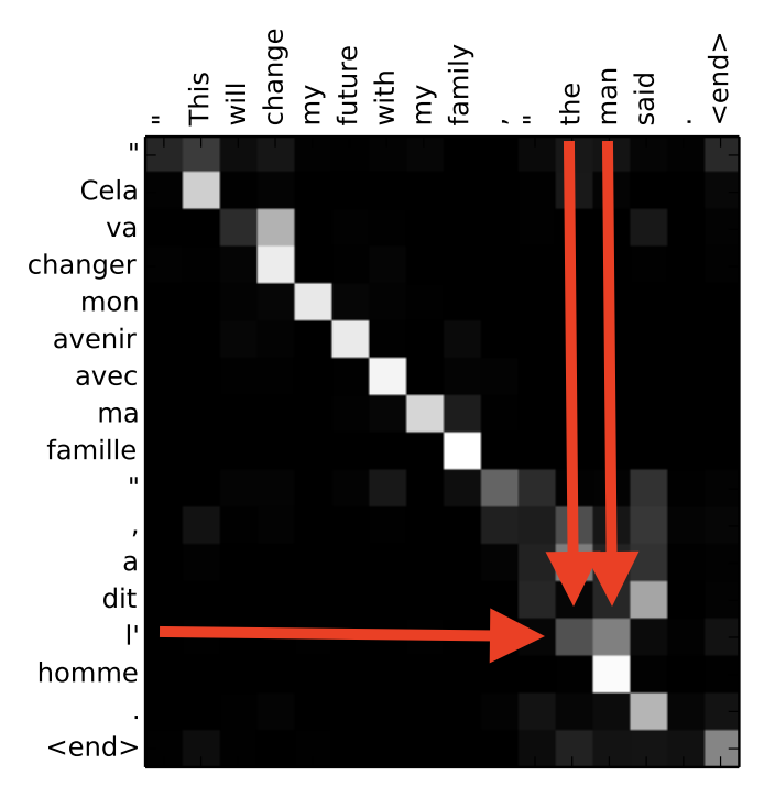
Figure 10 shows this behavior. The token l’ (a definite article meaning “the” that serves as a short form for masculine “le” and feminine “la”) attends to both “the” and “man” in the English sentence. Its connection to “the” is intuitive, while its connection to “man” highlights the fact that l’ hides this gender on its own and the surrounding noun remains essential to resolving the full meaning of the phrase.
Building on that encoder-decoder lineage, the Transformer kept a similar architecture but made attention the central mechanism for drawing global dependencies within the source and target sequences, and between them, as shown in Figure 11. Its encoder stack contains self-attention sublayers that process the source sentence. Its decoder stack uses two forms of attention: self-attention over the translation, and encoder-decoder attention over the final output of the encoder stack.
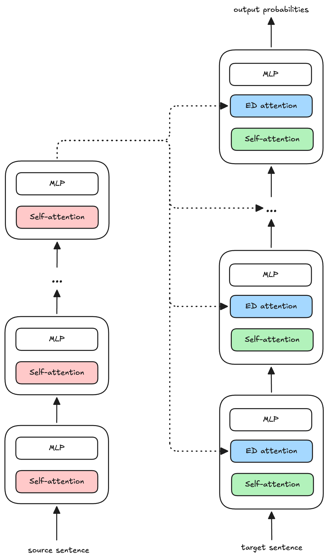
Later research found that, for monolingual text-to-text tasks, dropping the encoder and keeping only a stack of decoder blocks could simplify optimization and handle longer sequences more effectivelySee Peter J. Liu et al., “Generating Wikipedia by Summarizing Long Sequences” (arXiv, 2018).. That decoder-only model also exhibited an unexpected capability: although trained to generate Wikipedia articles, it learned to translate some names from English into other languages. GPT-2's authors later cited this behavior as an inspiration for their work, and GPT-2 continued the same broad decoder-only architecture and causal self-attention while making a few adjustments of its own.
Attention in GPT-2
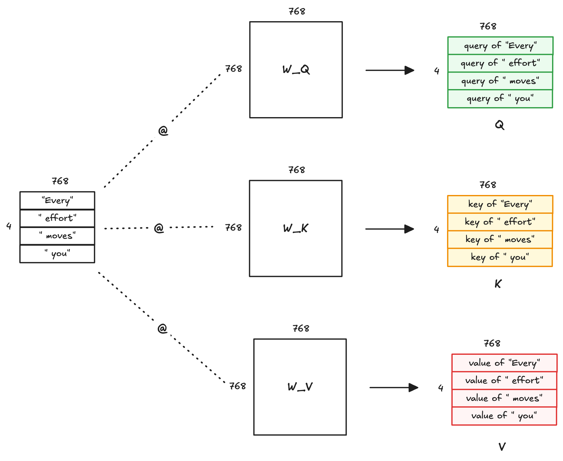
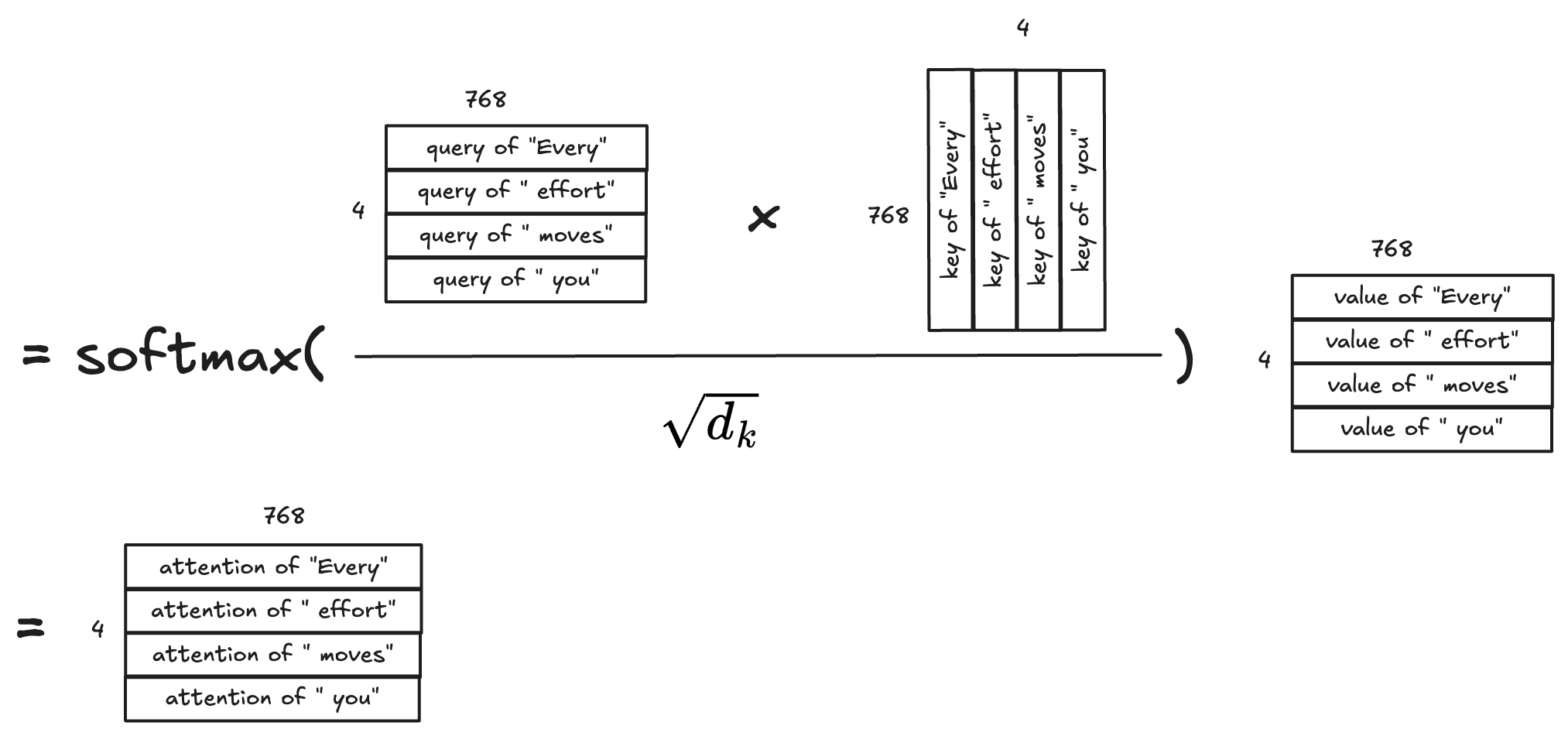
Inside attention, each token vector gets projected into three vectors: a query ($q$), a key ($k$), and a value ($v$). Each projection multiplies the token's current vector by a trained weight matrix and adds a learned bias. Figure 12 shows the matrix multiplications for the four-token sequence “Every effort moves you,” omitting the biases from the diagram:
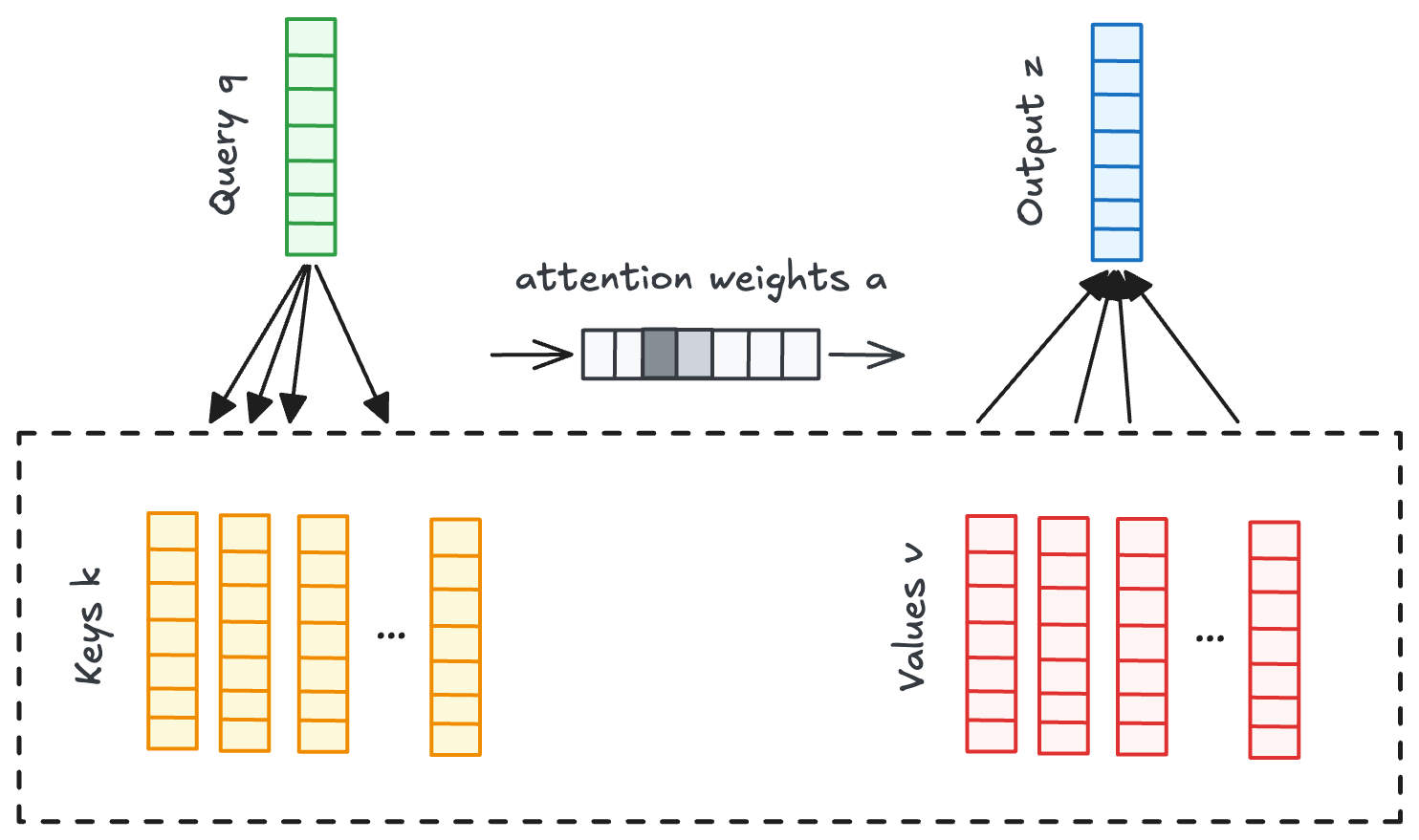
The roles of $Q$, $K$, and $V$ are similar to a dictionary lookup in a programming language such as Python, but the lookup is soft. A dictionary stores keys and their corresponding values, while a query specifies what to look up. As shown in Figure 13, attention takes the dot productThe dot product multiplies corresponding components of two vectors and sums the results into a single scalar. It can be interpreted as a similarity measure: the higher the score, the more similar the vectors are. between the query vector and each key vector, producing one score per key. Softmax then normalizes those scores into weights that add up to 1, called attention weights. Finally, attention takes the weighted sum of the corresponding value vectors to produce the output. As certain query-key dot products grow relative to the others, the combined attention weight assigned to those keys approaches 1, so the operation increasingly resembles retrieving a weighted combination of their values.
Attention equation
The equation for finding those scores is:
Scaling up the key-vector dimension $d_k$ can produce larger dot products that push softmax probabilities to extremes: the largest approaches 1, while the rest approach 0. In this saturated state, softmax gradients shrink toward zero, slowing or stopping weight updates. To avoid this kind of training instability, the scores are scaled by dividing them by the square root of the key-vector dimension:
These scaled scores are then passed through softmax, which normalizes the scores for each query into attention weights that add up to 1:
To produce the outputs (one per query), attention takes the weighted sum of the corresponding values:
Figure 14 visualizes the full operation:
Causal attention
The attention equation above lets each query attend to every token in the sequence, including those that come later. During training, GPT-2 uses the representation at each position to predict the following token. If that representation could already incorporate the following token's embedding, the answer would leak into the prediction. To prevent this, attention scores for later positions are masked by setting them to negative infinity ($-\infty$) before softmax, as shown in Figure 15.
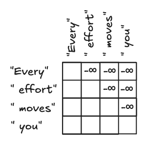
Since $\operatorname{softmax}(-\infty)=0$, masked positions receive zero probability, forcing each token to only look at itself and the tokens preceding it. With the future tokens masked, GPT-2's attention equation becomes:
Multiple heads
The relationship between tokens within a text is often multidimensional: grammar, meaning, and long-distance dependencies can all matter at the same time. To better capture this kind of multidimensionality, the model projects each token vector into several learned lower-dimensional subspaces, or heads, and performs attention in parallel within each one. Each head gets its own $W_Q$, $W_K$, and $W_V$ matrices and follows the independent attention operation explained above. This expands the model's ability to focus on different positions and relationships.
GPT-2 has 12 heads, each outputting a 64-dimensional output vector for each token. Those 12 vectors are then concatenated along the feature dimension to recover one 768-dimensional vector, then mixed by an output projection $W_O$:
Now you know what it means when you read that GPT-2 has a multi-head causal self-attention. “Self” means queries, keys, and values all come from the same sequence. “Causal” means the mask prevents reading future positions. “Multi-head” means the operation is repeated over several learned subspaces.
How GPT-2 learns
The perceptron at the beginning of this post learned by turning prediction errors into weight updates. GPT-2 does the same basic thing at a much larger scale during training: a forward pass produces logits, a loss measures the error, backpropagation traces that error to every parameter, and an optimizer updates those parameters. During inference, the resulting parameters remain fixed.
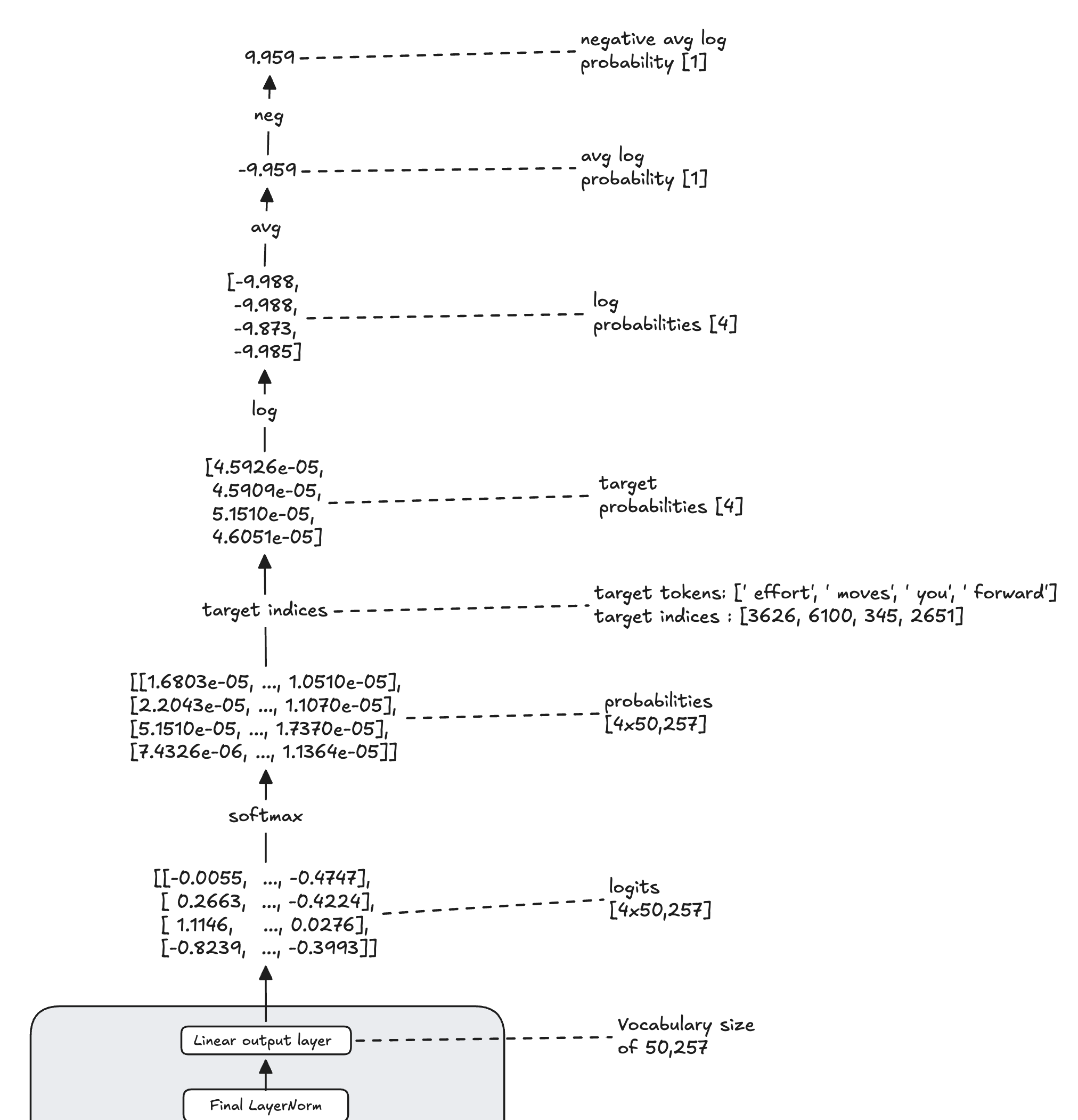
For the input “Every effort moves you,” Figure 7 shows GPT-2 producing a $4 \times 50{,}257$ tensor of logits. As shown in Figure 16 below, softmax converts each row into a probability distribution whose 50,257 values sum to 1, preserving the tensor's shape. The training step then uses the target indices $[3626, 6100, 345, 2651]$, corresponding to “ effort,” “ moves,” “ you,” and “ forward,” to select one probability from each row. For example, target index 2651 selects the value $4.6051 \times 10^{-5}$ from the fourth row. Such selected values form a target-probability vector with shape $[4]$. The loss calculation takes the logarithm of each target probability, averages the four log probabilities, and negates the result. Minimizing this negative average log probability, which is GPT-2's main training objective, pushes the target probabilities toward 1: $-\log(1)=0$.
During the forward pass, the operations that produced the loss are recorded in a computation graph. Backpropagation traverses that graph in reverse, applying the chain rule through the output projection, decoder blocks, and embedding tables. The result is a gradient for every trainable parameter: a measurement of how a small change to that parameter would change the loss.
The gradient provides a raw downhill direction; the optimizer decides how to scale and combine that information across training steps. That choice can determine how efficiently a training run converges. The field is therefore full of proposed improvements and a “graveyard of dead optimizers”See Keller Jordan, “Muon: An optimizer for hidden layers in neural networks” (Keller Jordan blog, 2024).. Below, I'll start with a one-dimensional slope, then trace the progression of optimizers that were adopted over time—from gradient descent and momentum through Adam and AdamW—before turning to newer methods such as Muon.
The Precalculus View
Imagine you are blindfolded, dropped somewhere on a mountainous landscape, and your goal is to find the absolute lowest point in the valley.
In machine learning:
- Your location on the map represents the model's current "weights" (its internal settings).
- Your altitude is the "Loss" (how wrong the model's predictions are).
- The lowest point is where the Loss is minimized.
In precalculus, if you have a simple curve like a parabola (a 2D valley), say $y = x^2$, you can look at the slope.
- If the slope is positive (uphill to your right), you must step left to go lower.
- If the slope is negative (uphill to your left), you must step right.
If you just feel the ground with your foot, determine the slope, and take a step in the opposite direction of the uphill slope, you will eventually reach the bottom.
As an update rule, that looks like this:
- $w_{t-1}$ is your current one-dimensional location.
- $y'(w_{t-1})$ is the slope of the curve at that location.
- $\alpha$ is the Learning Rate (how big of a step you take).
- The negative sign means you move in the opposite direction of the uphill slope.
Calculus & SGD (Stochastic Gradient Descent)
Calculus provides a mathematical tool called the derivative, which gives the exact slope at any given point. In 3D (or multi-dimensional) spaces, the analogous object is a vector of derivatives called the Gradient, usually represented by $\nabla$. The gradient always points in the direction of the steepest ascent (uphill).
To go downhill, step in the opposite direction: $-\nabla$.
This gives the rule for Gradient Descent:
- $w$ represents your weights (your coordinates).
- $L$ is the Loss function (altitude).
What makes it Stochastic (SGD)? Calculating the exact gradient using the entire training dataset at every update is too expensive. So, the optimizer estimates the gradient using a tiny, random sample of training examples (a "batch"). Because it's an estimate, the path is noisy and zigzaggy—like a drunken person stumbling down a hill—but it's computationally fast and gets you to the bottom eventually.
The "Ravine" Problem & Momentum
SGD has a fatal flaw. Imagine you are in a long, narrow ravine that slopes gently downwards toward the end, but has steep walls on the sides.
The desired direction is forward along the valley floor. But if SGD drifts even slightly left or right, the steep side-wall slope dominates the gradient. A large step then shoots it across the center toward the opposite wall, so it zigzags left and right while making slow forward progress.
The Fix: Momentum. Momentum adds a memory of past steps. Just like a heavy bowling ball rolling down a hill, the optimizer builds up speed in the directions that are consistent (down the valley) and cancels out the directions that alternate (bouncing left and right).
Adam (Adaptive Moment Estimation)
By 2014, researchers realized optimization could do better than just momentumDiederik P. Kingma and Jimmy Ba introduced Adam in "Adam: A Method for Stochastic Optimization".. In a neural network with billions of parameters, some parameters need huge adjustments, while others (which look at rare features) need very delicate, tiny adjustments. A single global learning rate ($\alpha$) isn't enough.
Adam was born. It tracks two things for every single parameter independently:
- The First Moment ($m_t$): an exponential moving average of gradients.
- The Second Moment ($v_t$): an exponential moving average of the squared gradients.
More precisely, Adam updates those two moment estimates, bias-corrects them, then uses them to update the weights:
Where:
- $g_t$ is the current gradient.
- $\hat{m}_t$ is the bias-corrected version of $m_t$.The bias comes from initializing $m_0$ at zero. Early $m_t$ values are pulled toward zero unless divided by $1 - \beta_1^t$. The same correction applies to $v_t$.
- $\hat{v}_t$ is the bias-corrected version of $v_t$.
- $\alpha$ is the learning rate.
- $\beta_1$ is usually $0.9$.
- $\beta_2$ is usually $0.999$.
- $\epsilon$ is a tiny stabilizing constant, usually $10^{-8}$, that prevents division by zero.
AdamW (Fixing Weight Decay)
Adam was the default for years, but it exposed a subtle issue with the usual way people applied regularization (specifically $L_2$ regularization)Regularization is a method used in neural networks to prevent overfitting by adding a cost term to the loss function. Common forms include L1 and L2.. For plain SGD, $L_2$ regularization behaves like weight decay, which means shrinking the weights slightly toward zero at every step. For Adam, that equivalence breaks because Adam adaptively rescales the gradient individually. For this reason, AdamW (Adam with Decoupled Weight Decay)Ilya Loshchilov and Frank Hutter introduced decoupled weight decay in "Decoupled Weight Decay Regularization". applies weight decay as a separate shrinkage step.
AdamW is the default standard today.
Using $\lambda$ for weight decay, AdamW writes the separate shrinkage directly into the weight update:
- The shrinkage term $(1 - \alpha\lambda)w_{t-1}$ is separate from the Adam update.
Muon (The Cutting Edge)
Muon (Momentum Orthogonalizer)See Keller Jordan, "Muon: An optimizer for hidden layers in neural networks", and Liu et al., "Muon is Scalable for LLM Training", which makes updates to it and proves that it works at large scale training. is an optimizer released in 2024 for matrix-shaped hidden-layer parameters. It forces the gradient update matrix to treat all directions more equally by replacing it with the nearest orthogonal matrix before applying the step.
Imagine a 2D plane. A vector is an arrow pointing in a specific direction with a specific length. Two vectors are orthogonal if they are perfectly perpendicular to each other, meeting at a 90-degree angle. The mathematical test is the dot product: if $\vec{A} \cdot \vec{B} = 0$, the vectors are orthogonal.
Geometrically, if you are walking strictly along Vector A (say, North), you are making zero progress in the direction of Vector B (East). Orthogonal vectors represent completely independent, non-overlapping directions or "concepts."
A matrix can be understood as an action on a vectorFor a visual explanation, see 3Blue1Brown, "Linear transformations and matrices".. An orthogonal matrix is a transformation that preserves the vector's geometry: it can rotate or reflect the vector, but it does not stretch, squash, or distort it. Lengths and angles are preserved, so all directions are treated equally.
Going back to the North/East example, a normal matrix might stretch the North direction by 10x, squash the East direction to 0.1x, and mix the diagonal direction unpredictably. An orthogonal matrix does not do that: it preserves every direction's scale relative to the others.
Coming back to Muon, it replaces the raw update with the nearest orthogonal matrix before applying the update, making the step more geometrically balanced. More concretely:
- $w_t$ is a matrix-shaped weight parameter.
- $g_t$ is its gradient matrix.
- $\mu$ is the momentum coefficient.
- $u_t$ is the momentum-smoothed update matrix.
- $o_t$ is the nearest orthogonal or semi-orthogonal version of $u_t$, approximated in practice with Newton-Schulz iterationSee "Muon Optimizer Explained", step 6..
How GPT-2 generates text
Training gives GPT-2 fixed parameters. To generate text, it processes the prompt, selects a next token, appends that token to the sequence, and predicts again. The initial prompt pass is called prefill; the one-token-at-a-time loop that follows is called decode.
During prefill, every decoder block computes a key and value vector for each prompt token. At a decode step, the new token's query must attend to those earlier keys and values. Recomputing all of them after every new token would repeat work whose inputs have not changed, so the model stores them in a key-value (KV) cache. Each step computes and appends only the new token's keys and values, then attends over the stored history.
The cache trades repeated computation for memory: it grows with context length, layer count, and the number and size of key-value heads. That tradeoff is why modern architectures care about key-value heads and attention span. The next section returns to GPT-2's decoder block and asks how newer models add capacity, use longer contexts, and control this growing cost.
From GPT-2 to modern LLMs
Modern LLMs still use GPT-2's basic loop: attention moves information between tokens, an FFN transforms each token, residual connections carry the representation forward, and the stack predicts the next token. What changed is the scale—more capacity and longer contexts—and the architectural choices needed to keep larger models trainable and affordable to serve.
I'll focus on high-level model-architecture changes. The table summarizes the main differences between GPT-2 and representative modern LLMs, and the following sections explain those changes in more detail.
| Component | GPT-2 | Representative modern choices |
|---|---|---|
| Scale | Up to 1.5B dense parameters | Much larger dense models, or sparse models with far more total than active parameters |
| Position information | Learned absolute embeddings | RoPE, or occasionally no explicit positional encoding |
| KV representation | One key-value head per query head | Shared key-value heads with GQA, or a compressed latent representation with MLA |
| Attention span | Full causal attention | Full attention, local windows, or alternating local and global layers |
| Feed-forward network | One dense GELU FFN per block | Dense SwiGLU FFNs, sparse MoE FFNs, or a mixture of dense and MoE layers |
| Normalization formula | LayerNorm | Often RMSNorm |
| Normalization placement | Pre-Norm | Pre-Norm, or both Pre- and Post-Norm |
| Vocabulary | 50,257 tokens | Often larger and designed for more languages |
| Residual width | Up to 1,600 dimensions | Often wider, alongside more layers and larger FFNs |
More capacity
Some SOTA models use a technique called Mixture-of-Experts (MoE) to increase their parameter count by 100x-1000x over GPT-2 XL—and therefore their capacity to store information and learn complex patterns—while increasing per-token computation by a much smaller factor. An MoE layer replaces an FFN within a decoder block with a set of FFNs called experts. A small router scores the experts for each token, then sends the token through only one or a few of the highest-scoring experts. This sparse routing largely decouples total parameter capacity from per-token computation, allowing the model to expand its capacity without making inference unbearably slow.
Expert designs vary. DeepSeekMoE divides the FFN capacity into many smaller experts and adds an always-active shared expert. The architecture is designed so the shared path can absorb broadly useful computation, reducing redundancy among the routed expertsSee Damai Dai et al., “DeepSeekMoE: Towards Ultimate Expert Specialization in Mixture-of-Experts Language Models” (arXiv, 2024).. Dense and MoE FFNs can also coexist: a model may alternate dense and sparse layers or keep an always-active path inside each MoE block.
Longer contexts
GPT-2 uses learned absolute positional embeddings. Because its positional embedding table contains only 1,024 rows, it has no embedding to assign to token 1,025. Most modern LLMs address this limitation with techniques such as Rotary Position Embeddings (RoPE)See Jianlin Su et al., “RoFormer: Enhanced Transformer with Rotary Position Embedding” (arXiv, 2021)., which rotate each query and key according to its position. Their dot product then depends on relative displacement, providing relative-position information without a fixed positional lookup table and making it possible to extend models to much longer sequences. Some models instead omit explicit positional encoding altogether. Experiments with NoPE show that useful position-dependent patterns can emerge implicitly from the causal structureSee Amirhossein Kazemnejad et al., “The Impact of Positional Encoding on Length Generalization in Transformers” (arXiv, 2023)..
During inference, the model must store the keys and values of every previous token in GPU memory—the KV cache—to generate the next token. In GPT-2's design, this cache grows linearly with batch size and context length, and also with layer count and the number and size of key-value heads, so long contexts can quickly exhaust available VRAM.
Attention variants such as Grouped-Query Attention (GQA) and Multi-head Latent Attention (MLA) address this memory constraint in different ways. GPT-2's multi-head attention gives every query head its own key and value head. GQA keeps the full set of query heads but lets groups of them share key and value headsSee Joshua Ainslie et al., “GQA: Training Generalized Multi-Query Transformer Models from Multi-Head Checkpoints” (arXiv, 2023).. If a layer has 32 query heads and 8 key-value heads, each KV head serves four query heads, making the KV cache four times smaller than it would be with 32 key-value heads. MLA instead compresses the key-value information into a low-dimensional latent representation that is cached and later used to derive the required keys and valuesSee DeepSeek-AI, “DeepSeek-V2: A Strong, Economical, and Efficient Mixture-of-Experts Language Model” (arXiv, 2024).. GQA reduces the cache through head sharing; MLA reduces it through compression.
Attention span is a separate choice. Full causal attention lets a query inspect every earlier position. Sliding-window attention restricts it to a fixed relative window, reducing the work at that layer. A model can combine a local window with MHA or GQA because the window decides which positions are visible while the head arrangement decides how keys and values are represented. Mistral 7B, for example, combines sliding-window attention with GQASee Albert Q. Jiang et al., “Mistral 7B” (arXiv, 2023).; other models alternate local and global layers.
Making decoder blocks easier to train and more effective
Scaling GPT-2 means repeating the same decoder block many more times, so small problems inside the block compound. Modern architectures simplify normalization to reduce unnecessary computation, place it where gradients remain well behaved, and use gated FFNs to control feature flow more expressively. RMSNorm, revised normalization placement, and SwiGLU address these problems in different ways.
LayerNorm subtracts the feature mean and divides by the standard deviation. RMSNorm skips the mean subtraction and divides by the root mean square insteadSee Biao Zhang and Rico Sennrich, “Root Mean Square Layer Normalization” (NeurIPS, 2019).. Its calculation is simpler, and it has worked well enough in large language models to become a common replacement for LayerNorm.
GPT-2 normalizes a vector before the attention module or FFN—an arrangement called Pre-Norm—then adds the module's output to the residual streamSee Ruibin Xiong et al., “On Layer Normalization in the Transformer Architecture” (ICML, 2020).. Some models instead add the module's output to the residual stream and normalize the sum—Post-Norm—while others use both placements. Gemma 2, for example, applies RMSNorm to the input and output of each attention module and FFNSee Gemma Team, “Gemma 2: Improving Open Language Models at a Practical Size” (arXiv, 2024)..
GPT-2's FFN uses one input projection followed by GELU. A SwiGLU FFN uses two input projections: one passes through SiLU and acts as a gate, while the other carries the values. Their element-wise product is projected back to the residual widthSee Noam Shazeer, “GLU Variants Improve Transformer” (arXiv, 2020).:
The second input projection adds parameters, so SwiGLU models commonly use a narrower intermediate layer than GPT-2's $4\times$ expansion. The same gated FFN can be used as each expert inside an MoE layer.
A modern LLM is therefore still recognizably GPT-like. The important changes are economic: sparse FFNs add stored capacity without using all of it for each token, GQA and MLA reduce cache memory, local attention limits how many positions some layers inspect, and revised normalization and gating make the repeated block more effective.
Conclusion
The history of AI shows us that what is hard for humans is often easy for computers, while what feels easy to us is often hard for them. Computers mastered formal tasks such as arithmetic and chess long before they could reliably recognize a face, understand speech, or use language. One successful solution to these intuitive problems is deep learning in general and large language models in particular.
Two key features separate these systems from many of their predecessors. First, they learn the representation itself rather than relying on hand-designed features. Second, they compose these representations across many layers, allowing them to “understand the world in terms of a hierarchy of concepts, with each concept defined through its relation to simpler concepts”See Ian Goodfellow, Yoshua Bengio, and Aaron Courville, “Deep Learning” (MIT Press, 2016)..
In this sense, GPT-2 was a small system with a spark. Today's state-of-the-art base models are recognizably the same kind of system under the hood, with greater scale plus architectural refinements making them far more capable. As mentioned at the beginning, modern LLMs also go through a post-training stage that shapes a pretrained model so its powerful capabilities are easier to steer and use.